23. Excel tools
In Excel, think-cell adds ribbon commands that make it easier to prepare and format your data before you present it in PowerPoint using think-cell elements. These think-cell tools are also useful independently in Excel.
The built-in Excel rounding tool can make the result of calculations appear incorrect, because Excel can only consider each cell value individually. The think-cell 23.2 Excel data rounding functions consider calculations holistically and round in such a way that the deviation from the precise values is minimal while keeping the calculation correct using the rounded values, where this is mathematically possible.
think-cell also allows you to apply table styles defined in Excel as regular formatting with a single click to a selected range of cells, without turning that range into a table. See 23.4 Applying Excel table styles as regular formatting.
23.1 The think-cell ribbon in Excel
After installing think-cell, you can use think-cell commands on the Excel ribbon.
The think-cell ribbon tab contains think-cell and Excel commands organized from left to right to reflect the process of working with data.
If you don't see the think-cell tab, your organization may have its own ribbon configuration and can provide related support. In many cases, you can go to Insert > think-cell to find frequently used think-cell commands. The Formulas tab may also contain think-cell commands.
You can customize the think-cell ribbon in Excel. For more information, see the following topics:
- Customize the think-cell tab (Windows only)
- Remove the think-cell tab
- Customize the ribbon in Office (Microsoft Support)
23.2 Excel data rounding
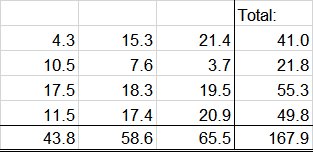
When data is compiled for a report or PowerPoint presentation, rounding summations in Excel is a frequent problem. It is often desirable, but difficult to achieve, that rounded totals exactly match the total of the rounded addends. For example, consider the following table:
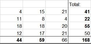
When the values are rounded to integers using Excel’s Format-Cell function, the following table results. Totals which appear to be “miscalculated” are in bold:
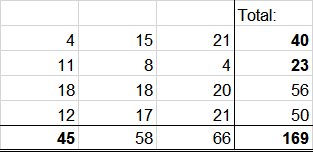
Similarly, when Excel’s standard rounding functions are used, totals of the rounded values are calculated correctly but rounding errors accumulate and results often deviate substantially from the actual totals of the original values. The following table shows the result of =ROUND(x,0) for the example above. Totals that deviate from the original value by 1 or more are in bold:
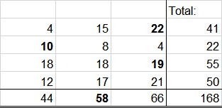
Using think-cell round, you can achieve consistently rounded totals with minimal “cheating”: While most values are rounded to the nearest integer, a few values are rounded in the opposite direction, thus maintaining correct calculations without accumulating rounding error. Since there are many possibilities to achieve correctly rounded totals by changing values, the software picks a solution that requires the minimum number of values changed and the minimum deviation from the precise values. For example, rounding down 10.5 to 10 is preferable over rounding down 3.7 to 3. The following table shows an optimal solution for the above example, with “cheated” values in bold:
To achieve this output in your own calculation, simply select the concerned range of Excel cells. Then, click the 
23.2.1 Using think-cell round
think-cell round seamlessly integrates into Microsoft Excel, providing a set of functions that are similar to Excel’s standard rounding functions. You can easily apply these functions to your own data using the think-cell round ribbon group in the Formulas tab.
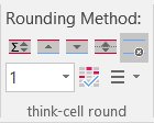
Rounding parameters
Like the Excel functions, the think-cell rounding functions take two parameters:
|
x |
The value that is to be rounded. This can be a constant, a formula or a reference to another cell. |
|
n |
The rounding precision. The meaning of this parameter depends on the function you use. The parameters for the think-cell functions are the same as for the equivalent Excel functions. Refer to the table below for examples. |
think-cell round can not only round to integer values, but to any multiple. For example, if you want to represent your data in 5-10-15-... steps, simply round to multiples of five. Using the dropdown box in the think-cell round toolbar, simply type in or select the desired rounding precision. think-cell round chooses the appropriate function and parameters for you. The following table provides some examples of rounding certain x-values using the toolbar together with their specific n-parameter.
|
x =
n =
|
100 |
50 |
2 |
1 |
0.01 |
|---|---|---|---|---|---|
|
1.018 |
0 |
0 |
2 |
1 |
1.02 |
|
17 |
0 |
0 |
18 |
17 |
17.00 |
|
54.6 |
100 |
50 |
54 |
55 |
54.60 |
|
1234.1234 |
1200 |
1250 |
1234 |
1234 |
1234.12 |
|
8776.54321 |
8800 |
8800 |
8776 |
8777 |
8776.54 |
If the values are not displayed the way you expect them to, verify that the Excel Cell Formatting is set to General and the columns are wide enough to display all decimal places.
|
Button |
Formula |
Description |
|---|---|---|
|
|
|
Let think-cell round decide to which of the two nearest multiples to round to minimize rounding error. |
|
|
|
Force rounding of x away from zero. |
|
|
|
Force rounding of x towards zero. |
|
|
|
Force rounding of x to the nearest multiple of the desired precision. |
|
|
Remove all think-cell round functions from the selected cells. |
|
|
|
Select or type the desired rounding multiple. |
|
|
|
Highlight all cells which think-cell decided to round to the farther of the two closest multiples instead of to the nearest. |
For optimal results with as little deviation from the underlying values as possible, you should use TCROUND wherever possible. Only use the more restrictive functions TCROUNDDOWN, TCROUNDUP or TCROUNDNEAR if you must.
Attention: You should never use nondeterministic functions like RAND() within any of the TCROUND formulas. If functions return a different value every time they are evaluated, think-cell round will make mistakes calculating values.
Layout of the calculation
The rectangular layout of the example above is only for sake of demonstration. You can use the TCROUND functions to determine the display of arbitrary summations spread across your Excel sheet. Excel’s 3-D references to other sheets and links to other files do also work.
Placement of TCROUND functions
Since TCROUND functions are meant to control the output of a cell, they must be the outermost function:
|
Bad: |
|
|
Good: |
|
|
|
|
|
Bad: |
|
|
Good: |
|
If you happen to enter something along the lines of the bad examples, think-cell round will notify you with the Excel error value #VALUE!.
23.2.2 Limitations of think-cell round
think-cell round always finds a solution for arbitrary summations with subtotals and totals. think-cell round also provides sensible solutions for some other calculations involving multiplication and numerical functions. However, for mathematical reasons, the existence of a consistently rounded solution cannot be guaranteed as soon as operators other than +, - and SUM are used.
Multiplication with a constant
In many cases, think-cell round produces good results when constant multiplication is involved, i.e., at most one of the coefficients is derived from the result of another TCROUND function. Consider the following example:

The precise calculation for cell C1 is 3×1.3+1.4=5.3. This result can be met by rounding up the value 1.4 to 2:

However, think-cell round can only “cheat” by rounding up or rounding down. Further deviation from the original values is not supported. Thus, for certain combinations of input values, no consistently rounded solution can be found. In this case, the function TCROUND evaluates to the Excel error value #NUM!. The following example illustrates an unsolvable problem:

The precise calculation for cell C1 is 6×1.3+1.4=9.2. Rounding cells A1 and B1 would result in 6×1+2=8 or 6×2+1=13. The actual result 9.2 cannot be rounded to 8 or 13, and the output from think-cell round looks like this:

Note: The Excel function AVERAGE is interpreted by think-cell round as a combination of summation and constant multiplication. Also, a summation where the same addend appears more than once is mathematically equivalent to a constant multiplication, and the existence of a solution is not guaranteed.
General multiplication and other functions
As long as the TCROUND functions are used for all relevant cells and intermediate results are connected merely by +, -, SUM and AVERAGE, the addends as well as (intermediate) totals are integrated into a single rounding problem. In these cases, think-cell round will find a solution that provides consistency throughout all cells involved, if such a solution exists.
Since TCROUND is a normal Excel function, it can be combined with arbitrary functions and operators. But when you use functions other than the ones mentioned above to connect results from TCROUND statements, think-cell round cannot integrate the components into one interconnected problem. Instead, the components of the formula will be taken as distinct problems which will be solved independently. The results will then be used as input to other formulas.
In many cases, the output from think-cell round will still be reasonable. There are cases, however, where the use of operators other than +, -, SUM and AVERAGE leads to rounded results which are far off from the result of the non-rounded calculation. Consider the following example:

In this case, the precise calculation for cell C1 would be 8.7×1.7=14.79. Since cell A1 and cell B1 are connected by a multiplication, think-cell round cannot integrate the formulas from these cells into a common problem. Instead, after detecting cell A1 as valid input, cell B1 is evaluated independently and the output is taken as a constant within the remaining problem. Since there are no further constraints, value 1.7 from cell B1 is rounded to the nearest integer, which is 2.
At this point, the “precise” calculation for cell C1 is 8.7×2=17.4. This is the problem that think-cell round now tries to solve. There is a consistent solution which requires rounding up 17.4 to 18. The result looks like this:

Note that the rounded value in cell C1, which is 18, greatly differs from the original value 14.79.
23.2.3 Troubleshooting TCROUND formulas
There are two possible error results you may come across when using think-cell round: #VALUE! and #NUM!.
#VALUE!
The #VALUE! error hints to syntactical problems, such as mistyped formulas or bad parameters. Also, pay attention to use correct delimiters: For example, while in the English version of Excel the formula looks like this: =TCROUND(1.7, 0), in a localized German version of Excel it must be written as =TCROUND(1,7; 0).
Another mistake specific to think-cell round is the placement of the TCROUND function call: You cannot use a TCROUND function within another formula. Please make sure that TCROUND is the outermost function of the cell’s formula. (see Placement of TCROUND functions)
#NUM!
The #NUM! error results from numerical problems. When the output of a TCROUND function is #NUM!, this means that the problem as stated by the given set of formulas is mathematically unsolvable. (see 23.2.2 Limitations of think-cell round)
As long as the formulas enclosed by TCROUND functions contain merely +, - and SUM, and all TCROUND statements share the same precision (second parameter), a solution is guaranteed to exist and will be found by think-cell round. However, in the following cases there is no guarantee that a consistently rounded solution exists:
- Formulas involve other operations like multiplication or numerical functions. Also, summations where the same addend appears more than once are mathematically equivalent to a multiplication.
- You use different precisions in the second parameter of the
TCROUNDfunction. - You make frequent use of the specific functions
TCROUNDDOWN,TCROUNDUPandTCROUNDNEAR.
You can try to restate the problem to get a consistent solution. Try the following:
- Use a finer precision for some or all
TCROUNDstatements. - Do not use
TCROUNDwith multiplication or numerical functions other than +, - andSUM. - Use the same precision (second parameter) for all
TCROUNDstatements. - Use
TCROUNDinstead of the more specific functionsTCROUNDDOWN,TCROUNDUPandTCROUNDNEARwherever possible.
23.3 Calculate the compound annual growth rate (CAGR)
The think-cell TCCAGR formula simplifies the calculation of the compound annual growth rate (CAGR). Use this function to quickly analyze business data over time. For more information on the CAGR, see Wikipedia.
23.3.1 Use the TCCAGR formula
- In Excel, enter your data in a range of cells in a single row or column.
-
In another cell, type
=TCCAGR(FIRST_CELL:LAST_CELL). ReplaceFIRST_CELLwith the first cell in your range, andLAST_CELLwith the last cell.Alternatively, to calculate the CAGR directly from the Excel ribbon, select the data range in a row, then select think-cell > Formulas > Insert CAGR
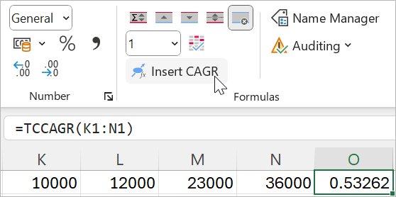
Note: The TCCAGR formula uses only the first and last cells in the range—the cells between the two do not affect the calculation. Furthermore, the formula requires positive values in both the first and last cells to return a meaningful result.
23.3.2 Represent a year in multiple cells
The TCCAGR formula has an optional second parameter to represent a year's data across multiple cells. To use this parameter, after the range, add the number of cells that represent a year. If you don't use this optional parameter, the TCCAGR formula takes each cell to represent one year by default.
For example: =TCCAGR(B1:B5) calculates the CAGR over a four-year period, with each cell representing one year. Using the optional parameter, =TCCAGR(B1:B9, 2) calculates the CAGR over a two-year period, with every two cells in the range representing one year.
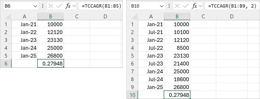
Note: Comma is used as the delimiter in most versions of Excel. In some localized versions, however, comma is the decimal separator, so the semicolon is used instead of the comma for parameters. Make sure to use the correct delimiter for your Excel version.
23.3.3 Troubleshoot the TCCAGR
There are three possible error results you may come across when using the TCCAGR formula: #VALUE!, #DIV/0!, and #NUM!.
#VALUE!
The #VALUE! error may result from mistyped formulas or bad parameters. Make sure to use the correct punctuation for localized versions. For example, in the English versions of Excel, the formula looks like this: =TCCAGR(A1:A10, 2), but in the German version of Excel, the comma is replaced with a semicolon: =TCCAGR(A1:A10; 2).
The TCCAGR formula works in a range of cells arranged in a single row or column. Using the formula with cells that are not in a single row or column will result in a #VALUE! error.
Another reason for a #VALUE! error is having a negative value in either the first or the last cell in the range. The TCCAGR formula requires positive numbers in both cells to function.
#DIV/0!
If the value of the first cell in the range is zero, the formula will return a #DIV/0! error, as the CAGR calculation would involve division by zero.
#NUM!
If both the first and the last cell in the range are zero, the formula will return a #NUM! error, as the TCCAGR requires both cells to have positive numbers.
23.4 Applying Excel table styles as regular formatting
Excel's Format as Table feature allows you to quickly transform a selected range of cells into a formatted table. However, this formatting is applied independently of regular cell formatting, and is therefore, for example, not recognized by VBA macros. Moreover, applying it is somewhat cumbersome, requiring at least three clicks.
think-cell allows you to define up to ten favorites and apply them to the selected range as regular cell formatting with a single click in the Ribbon.
To do so, first define the style you would like to apply:
- Go to Home>Styles>Format as Table and either:
- Create a completely new style by selecting New Table Style.
- Base your style on an existing one by right-clicking it and selecting Duplicate.
- Name the style "think-cell Table Style n" where n is a number from 1 to 10.
- Define the table formatting as usual and click OK.
Now you can add a button to the Ribbon that applies this table style as follows (see also C.6 Customize the think-cell ribbon):
- Right-click the Ribbon and select Customize the Ribbon.
- Select the tab you want to place the button on on the right, or create a new one by clicking New Tab.
- Create a new group in the tab by clicking New Group, or select an existing custom group.
- On the left, go to Main Tabs>think-cell Commands>think-cell Commands.
- Select think-cell Table Style n, where n is the number you picked in step 2.
- Click Add >>.

Repeat as needed for further table styles. The buttons placed in the Ribbon will show you a preview of the style that will be applied. You can also use the Rename button in the Ribbon customization dialog to give the buttons more descriptive names.
Note: The table style will always be applied with all header and total rows, first and last columns, and row banding defined. If you want a button for applying the table style without them, simply duplicate the style, change its name to a different n, and remove them. Column banding is not supported.
You can also place buttons for quick access to cell styles in the same way. Name them "think-cell style n" and place the corresponding think-cell Style button in the Ribbon.
Note: Custom table and cell styles are saved in the workbook, rather than globally in Excel. If you want to always use the same table styles assigned to the same buttons, create a workbook where those styles are assigned to the Ribbon buttons as described above, and save it as an Excel Template (*.xltx) that you use as a basis for future workbooks.
See here for general information on creating and using Excel templates.


