How to use Excel pivot tables for PowerPoint presentations

Pivot tables are so quick and powerful that they can seem almost magical to someone who discovers them for the first time. If you are used to writing formulas involving numerous COUNTIFS, SUMIFS, and INDEX MATCH functions, then you will instantly appreciate how easy it is to aggregate large volumes of data with Excel’s pivot tables.

What’s less easy is turning this aggregated data into an impactful chart for a presentation.

While Excel pivot tables are a great tool for data exploration, visualizing insights from pivot table data is fraught with challenges. Simply inserting a pivot chart from Excel into PowerPoint is possible, but it can lead to data and formatting inconsistencies. A specialized solution like think-will help maximize the impact of your analysis as part of a convincing presentation.

This article covers the following points:

• Benefits of working with Excel pivot tables for data exploration
• Common business use cases of Excel pivot tables
• Disadvantages of Excel pivot tables
• Visualizing your pivot table data in Excel and PowerPoint
• Recommended solution for visualizing pivot table data
• Two scenarios for creating charts from pivot tables for presentations
• Conclusion: bridging the gap from pivot table analysis to visualization
• Pivot table FAQ

---

If you’re new to think-cell and want to visualize your pivot table data more effectively in PowerPoint, you can download a free 30-day trial with unlimited access to all features:

Benefits of working with Excel pivot tables for data exploration

Pivot tables aren’t unique to Excel, but this article will focus on Excel, as it remains the most widespread tool for handling data in a business environment. Users can build pivot tables in Excel and analyze the data within the spreadsheet, and embed them in PowerPoint presentations.

If you are new to Excel Pivot tables, or you need a refresher on how to prepare and structure your data, then you can get a quick review on Microsoft’s support page.

The primary use of pivot tables is to convert large flat data tables, often with thousands of rows and dozens of columns, into a view with flexible column and row layouts that enables quick exploration and analysis. The pivot table makes it easy to run an ad-hoc analysis, exploring and slicing the data to discover insights that you wouldn’t otherwise have access to.

The advantages offered by pivot tables cover the whole process, from setting up the data to analyzing it and collaborating within teams.

Setting up the pivot table data

• Excel can parse any existing spreadsheet table, .txt or .csv file, and use it to generate a pivot table. You can export data from another tool, such as your inventory management software, Salesforce, Power BI, SAP or marketing analytics platforms, simply load it into Excel and create a pivot table.
• Excel reads the source data, but it doesn’t change it when creating a pivot table, so your input data remains clean and you don’t have to worry about inaccuracies.

Analyzing the pivot table data

• Pivot tables make raw data digestible by converting large datasets into smaller summary tables.
• Excel pivot tables only take a couple of clicks to set up so they are a quick way of conducting an ad-hoc exploration and get a first impression of a dataset.
• Excel lets you choose exactly which columns you want to include in your pivot table, which lets you simplify a dataset by focusing on relevant dimensions.
• Pivot tables do a lot of heavy lifting for you by automating aggregations that would otherwise require convoluted, error-prone formulas.
• Filters can be easily applied and edited, letting you hide less relevant data points and explore the data from different perspectives.
• Pivot tables can be easily refreshed to include any new or updated data,
• Excel lets you add slicers for filters and timelines for date-picking to make data exploration easier, even for users unfamiliar with the data set.

Collaborating within teams

• Pivot tables don’t require any programming knowledge of Python or SQL, or even Excel formulas, so non-specialists can easily work with them.
• Pivot tables in Excel are already embedded in the environment where many other business tasks take place, aiding file sharing, collaboration and connection to other spreadsheets
• Excel is fully compatible with other Microsoft Office programs so pivot tables can be easily copied and inserted into PowerPoint presentations or Word documents.
• Excel works with Power Query for teams with sophisticated requirements to build more complex data transformation pipelines that can feed into pivot tables.

Common business use cases of Excel pivot tables

Given the versality of Excel pivot tables, it’s not surprising that business professionals use them for a wide variety of use cases, as demonstrated by a selection of examples shared by knowledge workers:

• Simplifying large sets of data in a supply chain role
• Building reports from accounting software data exports
• Transforming data from SAP into a more manageable structure
• Creating weekly reports of quality issues
• Visualizing granular sales data by customer, item or region over time
• Preparing input data for use in other spreadsheets
• Summarizing large data sets in an accounting context
• Building reports that benefit from easy filtering and slicing

These use cases confirm two things. Firstly, pivot tables aren’t restricted to specific industries. Secondly, while pivot tables are often associated with ease of data exploration, making them well-suited to ad-hoc tasks and one-off analyses, pivot tables are also used as part of the process for generating recurring reports.

Disadvantages of Excel pivot tables

Pivot tables are a valuable tool for turning raw data into meaningful insights, as they help reveal patterns in datasets that would otherwise be too large to analyze. But Excel pivot tables do have some disadvantages, particularly for users who are less familiar with them:

• Referencing cells within pivot tables works differently from referencing standard Excel cells, which can lead to errors when making calculations that refer to pivot table data.
• Adding calculated rows or columns to pivot tables is a clunky experience, meaning that users often have to add helper columns to their source data.
• Preparing and cleaning your source data for a pivot table analysis can be a time-consuming process, unless the data originates as a standard export in a reliable format.
• Building dashboards is possible, but the functionalities of Excel pivot tables are very limited when compared to specialist business intelligence software like Tableau or Power BI.
• Refreshing has to be done manually and for each pivot table individually, which can lead to inconsistencies if source data has been refreshed.

As the primary purpose of pivot tables is data analysis, they have one clear disadvantage: they don’t easily allow for the creation of professional charts. The next section will look at how you can bridge the gap from a pivot table analysis to an impactful visualization that will support your storytelling.

Visualizing your pivot table data in Excel and PowerPoint

Powerful data visualization is essential for communicating messages effectively, but even rudimentary data visualization can also be a useful tool during data exploration. The starting point is the pivot table itself, which can already be considered a visualization of sorts. Small adjustments like changing number formatting, setting column widths, or displaying row and column totals can make it easier for you to digest the data and find insights.

The next level of sophistication, while still not going beyond the pivot table, is conditional formatting. Excel offers a range of conditional formatting options, which can be useful if applied effectively, but which can quickly get very messy, particularly if you restructure your data after having set up conditional formatting rules.

Creating a simple pivot chart from your pivot table

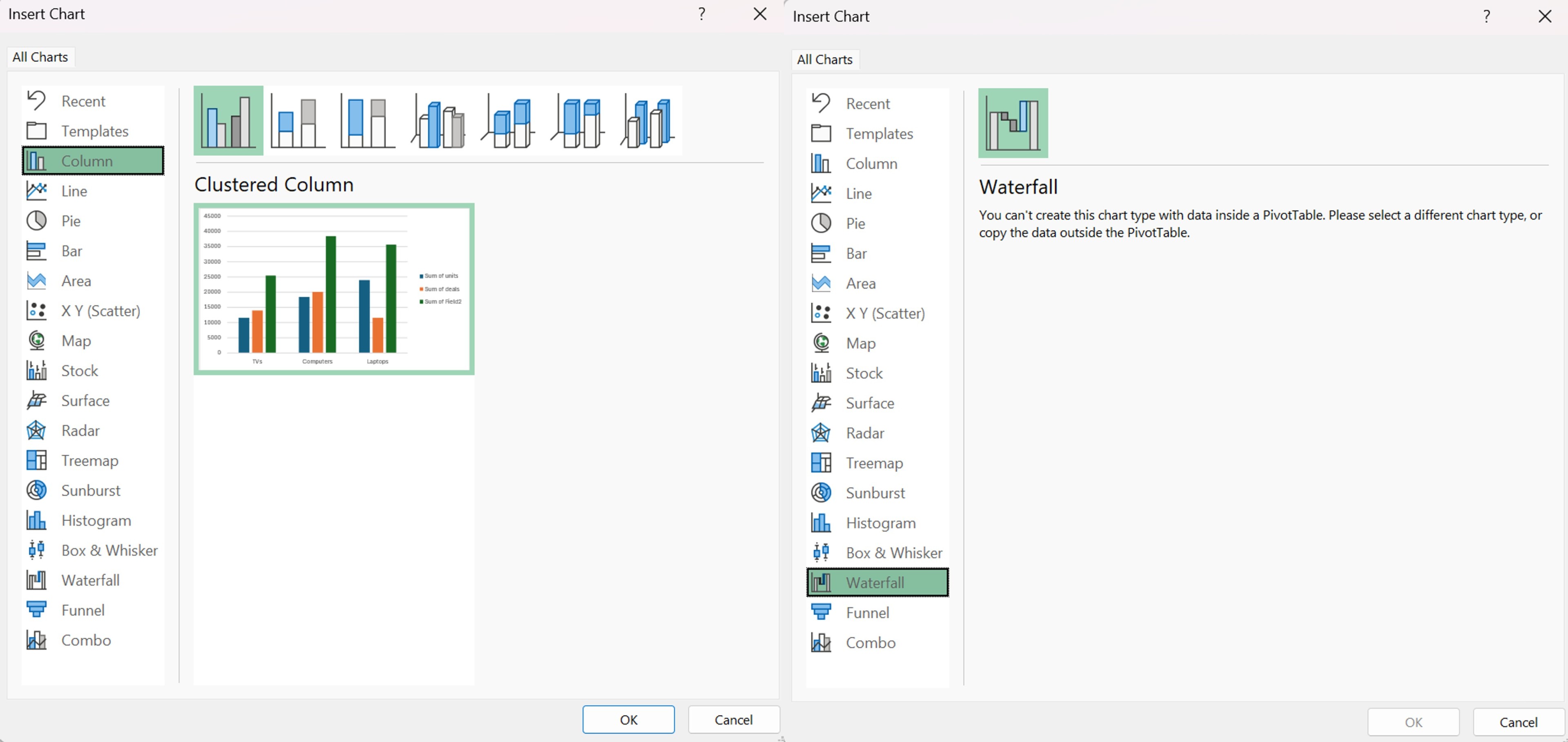
Even with conditional formatting, table visualizations can only go so far. Your best option for exploring your pivot table data is with a pivot chart, which you can easily insert by selecting PivotChart from the PivotTable Analyze tab in Excel. The dialog for inserting a pivot chart is the same as for other charts, albeit with some options (e.g., waterfall charts) not available for pivot table data.

---

Tip: Just like ordinary Excel tables, you can press Alt + F1 from within the pivot table to instantly create a pivot chart. This will be column chart by default, but you can easily right-click to change chart type and you can also adjust the formatting if needed.

---

Pivot charts look like other Excel charts, but they behave slightly differently, because they are tied to the data in your pivot table. Any updates to the pivot table will be automatically reflected in the chart, letting you instantly see how the data is impacted by changes you make to your columns, filters or data aggregations. Or if the pivot table data is refreshed, the pivot chart will refresh at the same time.

The link between the pivot chart and pivot table helps you analyze your data quickly and discover trends worthy of further exploration. And the link even works both ways, letting you make changes directly via the pivot chart that will be reflected in the pivot table.

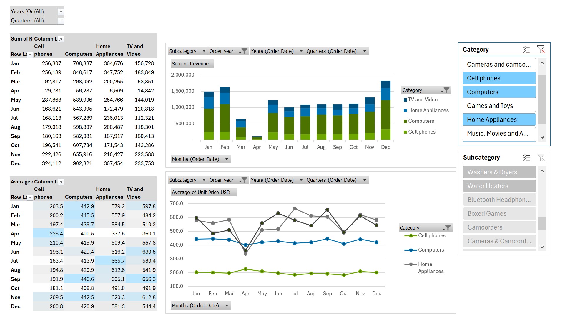
Building an interactive dashboard from pivot table data

By creating multiple pivot charts, you can use pivot tables to fuel interactive dashboards that let users explore the data from several angles at once. Filters can be used to control multiple charts simultaneously and reveal the relationships between different metrics or datasets.

While specialized business intelligence platforms like Tableau or Power BI exist for this purpose, it’s perfectly possible to use Excel to build attractive, functional dashboards with charts, tables, slicers, and timelines. Particularly for single-source data environments or for medium-sized businesses, Excel will often be the most suitable dashboard solution.

Whichever tool is used for the final output, pivoting the data in Excel can be a valuable way of quickly understanding its structure before setting up the data pipeline and building a complex dashboard.

Limitations of Excel pivot charts for presentations

Excel’s pivot charts essentially serve as an extension of the pivot table’s data exploration capabilities, rather than offering a robust data visualization experience. For all their value as a data exploration tool, Excel’s pivot charts are not often used in presentations, even though the functionality exists to copy them into PowerPoint. Reasons for this include:

• The data link between the pivot chart and the pivot table eliminates flexibility, meaning you have to remove a series from the table if you don’t want to display it in the chart.
• The pivot chart layout strictly follows the series and categories of the pivot table, which will often not be the layout you need. The only way to swap the series and columns in the pivot chart is to swap the rows and columns in the pivot table. This is rarely good for readability and it can sometimes break formulas by shifting or overwriting other elements on the Excel spreadsheet.
• Date grouping, such as by month or quarter, might be useful for understanding the data in the pivot table but it might not transfer to an attractive, readable chart.
• Number formats are not treated as part of the data link, so there can be misalignment between pivot chart labels and the data in the pivot table, which can cause confusion when switching between the two.
• The chart includes field, filter buttons and date grouping buttons that are useful for analyzing the data, but interfere with the visualization.

As well as these specific features of pivot charts, you still face all the other restrictions associated with formatting charts in Excel or PowerPoint. And many of these—such as clunky axis labelling—are only exacerbated by the fact that pivot table data often has a more complex structure than flat table data.

---

With think-cell Charts, it's easy to format and edit your charts so they're exactly how you need for your business presentations. You can download a free 30-day trial and start making impactful visualizations today:

Reference tables as a solution to pivot table limitations

A solution to the limitations of pivot charts is to decouple the pivot table data from the chart. Breaking the link between chart and table makes the pivot chart less useful for exploration, but it gives you more flexibility to make an impactful visualization.

When you set up a reference table, you have three options that can be useful depending on your scenario:

• Copy from the pivot table and paste values: Pasting values will capture the state of the pivot table at the moment you copy it. This can be a suitable approach if your data is finalized and you have settled on a view that you would like to visualize. It also means that you can continue to explore the data and change filters without your reference table changing.
• Reference the cells in formulas: Using formulas that refer to the cells in the pivot table will mean that your reference table will update if your pivot table data is refreshed, making it less prone to data inconsistencies. However, if you make changes to the structure of your pivot table, then your formulas may no longer reference the right cells. This is best if you have settled on a pivot table structure but expect the source data to be refreshed.
• Use GETPIVOTDATA: Working with the GETPIVOTDATA function lets you reference fields and items in the pivot table by name, so your formula doesn’t break even if the fields or items move as you restructure the pivot table. This is a powerful option but it requires more complex formulas and it can still result in errors depending on which changes are made to the pivot table data.

Whichever option you use, you will encounter the fewest errors if you complete your pivot table analysis before setting up your reference table. This isn’t always practically possible, but once you have the final data structure and number of series, and you know what you want to draw attention to, you can exercise much more freedom in your visualization.

Pivot tables don't refresh automatically when the source data changes, so always remember to refresh your pivot table, or your reference table won't be updated either.

Linking your Excel pivot table data to PowerPoint

With your reference table in place, you can use it as the source data for a chart, which you create and format in the usual way in Excel. To add the chart to a presentation, it’s easy to copy it from Excel into PowerPoint. The Paste Special tool provides a few methods to choose how you insert the chart into your presentation:

• Microsoft Excel Chart Object: Inserts a chart with a datasheet embedded in PowerPoint that lets you format the chart and edit data directly within the presentation.
• Linked Microsoft Excel Chart Object: Pastes a chart that’s linked to the source Excel file so that updates made in Excel will be reflected in the chart within the PowerPoint presentation.
• Picture (various formats): Creates an image (e.g., .jpg, .png) of the chart in its current formatting.

Each of these options has disadvantages to be aware of:

• Non-linked Microsoft Excel Chart Objects can be difficult to edit in PowerPoint, and they create a disconnect between the chart in your presentation and the data in your spreadsheet.
• Linked objects can lose the connection to the Excel file if the file is renamed or moved.
• Pictures are only viable if your chart formatting and data are completely finalized, as changes you make after pasting will not be reflected.

Knowing these drawbacks is a start to working around them, but they all mean that the standard link between your Excel pivot table and PowerPoint can lead to some kind of frustration.

Recommended solution for visualizing pivot table data

Whether you format your chart in PowerPoint or directly in Excel, and whether you embed the chart, paste a link or insert an image, you are still faced with a fundamental problem: you are using a data analysis tool for data visualization.

It’s always preferable to use specialist solutions for specialist tasks. So, you use an Excel pivot table for your data analysis and you use PowerPoint for your presentations, but for data visualization, you should really be using a purpose-built data visualization solution.

---

The think-cell Suite gives you everything you need to easily build professional charts from your pivot table data, including Excel links that are more stable and flexible than Microsoft’s standard offering. Try it for yourself in a free 30-day trial:

---

Creating reference tables when using think-cell

When you use think-cell, it’s still best practice to create a reference table to decouple the pivot table data for your analysis from the data for your chart. There is just a slight difference, as think-cell charts require a particular data layout. For example, if you’re building a think-cell column chart, you should include a second row for category totals.

For more information about ensuring your Excel data layout is set up for think-cell charts, see our user manual.

Two scenarios for creating charts from pivot tables for presentations

Just as pivot tables are used to generate insights in a wide range of business contexts, there are also few restrictions on how these insights are presented. To cover some of the most common cases, this section will address two general scenarios for visualizing and presenting pivot table data, and show how think-cell can help with this vital part of the decision-making process:

• Scenario 1: Connecting a pivot table to a recurring report in PowerPoint
• Scenario 2: Including pivot table data in an ad-hoc presentation

Scenario 1: Connecting a pivot table to a recurring report in PowerPoint

Pivot tables are widely used to create weekly or monthly PowerPoint reports that can be built once and simply refreshed with the new data. think-cell’s linking has two critical advantages that make automation of recurring reports from pivot tables more stable, efficient, and less susceptible to errors:

• Robust Excel links: The ordinary links from Excel to PowerPoint, generated when inserting a chart, will break if a file is moved or renamed. This can easily happen for recurring reports, particularly if new versions are saved for each iteration or they are shared amongst a broader team. think-cell Excel links are preserved even when a file is renamed, moved, sent as an email attachment, or even if the linked slide is copied to another file. Whatever happens, you never have to worry about the connection to your pivot table data being lost.
• Data links for text: think-cell links aren’t limited to charts or data tables. You can also link the value in an Excel cell to text in a PowerPoint shape or text box. This lets you reference totals or trends from your pivot table and include them in annotations that will automatically refresh in sync with your charts.

Note: While think-cell’s Excel links can be set to update automatically when the data changes, Excel’s pivot tables do not update automatically with the source data. Always check your pivot table is refreshed if you want your PowerPoint presentation to be correct.

Saving time and increasing accuracy of reports are clear primary benefits, but the secondary benefits are no less significant. With the menial aspects automated, teams have more mental capacity for analysis and ad-hoc observations. By enhancing their report with meaningful insights, they can create more value for the company, drive business decisions, and strengthen their own personal reputation.

Scenario 2: Including pivot table data in an ad-hoc presentation

One of pivot tables’ main strengths for data exploration is that they let the user set filters and choose the categories they want to look at. But this choice is precisely what you don’t want if you are controlling the narrative in an ad-hoc PowerPoint presentation. You want a fixed view of the data so that you can highlight your perspective and use it to support your arguments.

think-cell’s charting capabilities let you tell exactly the story you want, without compromises. You can read in detail about think-cell charts, but three features stand out when getting the most impact from your pivot table data for your ad-hoc presentation:

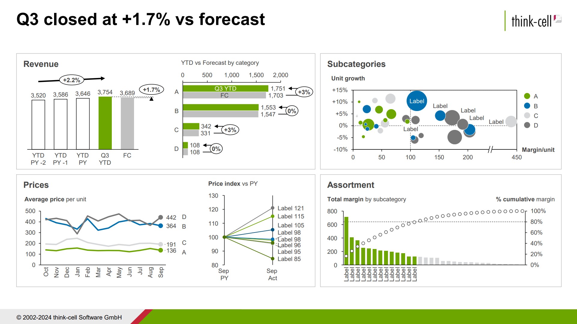
• Auto-calculated annotations: If your pivot table shows developments over time, there will often be one category with an interesting or unexpected trend you want to highlight. think-cell makes it easy to add auto-calculated growth rates or deltas that that visually emphasize the slide’s main takeaway and help tell your story.
• Waterfall charts: Pivot tables are often used to sum values by category, which can form the basis of a waterfall chart showing how each category contributes to an overall change. think-cell’s industry-leading waterfall charts are much more flexible than the standard options offered by Excel and PowerPoint.
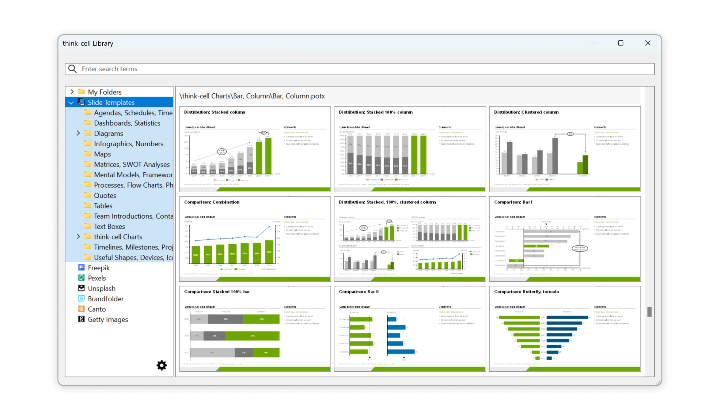
• Brand compliance: If you’ve run an ad-hoc analysis with a pivot table and you’re working at speed, then you don’t have time to worry about adjusting it to brand colors, fonts and styling. With the think-cell Library, you can easily access your company’s corporate templates. All you have to do is insert the chart into your presentation and you know that it will be on-brand and make a professional impression.

Conclusion: bridge the gap from pivot table analysis to visualization

Excel pivot tables are highly versatile for data analysis but you need a specialized tool to bridge the gap from exploration to visualization. The pivot table will help you draw powerful insights from a dataset but not communicate them effectively to your audience.

think-cell closes the loop by integrating seamlessly into Excel and PowerPoint and helping you bring your pivot table data to life. think-cell also equips you with tools for creating professional business slides that will help frame your charts and make your messages as impactful as possible.

If you haven’t tried it yet, you can download a free think-cell Suite trial today and get unlimited access to all features for a full 30 days:

Pivot table FAQ

This section answers some of the most frequently asked questions about working with pivot tables in Excel and PowerPoint.

What is a pivot table?

A pivot table is a tool for summarizing and analyzing large datasets by totaling, counting or otherwise aggregating values. For example, a pivot table can take a large quantity of sales data with individual line items and show totals grouped by product type, region and quarter. The term ‘pivot’ is used because the source data is not changed. It is simply turned around, grouped or viewed from a different perspective e.g., by converting a column heading into row labels.

How do you create a pivot table in Excel?

To create a pivot table in Excel, you first highlight your data range and select Format as Table from the Home tab. You can choose any formatting style you like but you should make sure your data has a header row as this will be needed for the pivot table.

Once table formatting is applied, you can select Summarize with PivotTable from the Table Design tab. Click OK and a new worksheet will be created with the pivot table field list in the right-hand sidebar. Here, you can select fields or drag them into the relevant areas to create your pivot table.

How do I insert a calculated field in a pivot table?

To insert a calculated field in a pivot table, you first select Calculated Field from the Fields, Items & Sets menu of the PivotTable Analyze tab. This opens the Insert Calculated Field dialog, where you can add the formula for your calculated field.

If you wish to reference existing fields, you can select them from the field list and use the Insert Field button. As a simple example, if you want to calculate the sum of two fields named Price and Tax, your formula should read =Price+Tax. You can enter a title for your calculated field by typing in the name. When you are finished, simply click Add and the calculated field should appear in your pivot table.

How can you remove zero values from a pivot table?

You can either remove zero values from the individual rows in the pivot table’s source data, or from the aggregated values (e.g., sums) in the pivot table itself.

To remove zero values from the source data, you can add a filter by dragging the relevant field into the Filters area in the field list in the right-hand sidebar. The filter menu will appear above the pivot table, by default in cells A1 and B1 of the worksheet. To remove zero values, you then open the dropdown menu in cell B1 (by default), check Select Multiple Items and then remove the check from 0, leaving all other values checked.

To remove any aggregated zero values from the pivot table, you click the filter symbol next to Row Labels in the top-left cell of the pivot table. By default this is cell A3 of the worksheet. You then select Value Filters > Does not equal, and type 0 where prompted by the dialog. Ensure that you choose the relevant field to filter from the drop-down menu.

How can I create a pivot table from multiple sheets?

To create a pivot table from multiple Excel sheets, you first go to a new sheet and select the PivotTable menu from the Insert tab. Here you choose From Data Model and click OK to specify where the pivot table should be inserted.

The top window of the right-hand sidebar will now list all the available tables in the Workbook’s data model. You can click any table to expand it and select which fields you want to add to your pivot table.

Creating a pivot table from tables on multiple sheets is most effective if the tables share an index or ID column that can be used to create a meaningful relationship between the tables.

How can I add a percentage to a pivot table?

You can add a percentage to a pivot table in many ways, but the most common reason to add a percentage to a pivot table is to display the values in a column as a percentage of the column total. For example, you may have total sales counts by product type and you want to see each total as a percentage of all sales.

To display the values as a percentage, you right-click on one of the values in the relevant column of your pivot table, and go to Show Values As in the context menu. From here, you have different options, such as % of Grand Total and % of Column Total, or you can choose % Of... and select the base field you want to reference.